SciPy - ODR

ODR stands for Orthogonal Distance Regression, which is used in the regression studies. Basic linear regression is often used to estimate the relationship between the two variables y and x by drawing the line of best fit on the graph.

The mathematical method that is used for this is known as Least Squares, and aims to minimize the sum of the squared error for each point. The key question here is how do you calculate the error (also known as the residual) for each point?

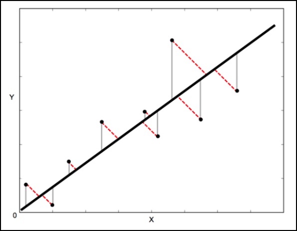
In a standard linear regression, the aim is to predict the Y value from the X value – so the sensible thing to do is to calculate the error in the Y values (shown as the gray lines in the following image). However, sometimes it is more sensible to take into account the error in both X and Y (as shown by the dotted red lines in the following image).

For example − When you know your measurements of X are uncertain, or when you do not want to focus on the errors of one variable over another.

Orthogonal Distance Regression (ODR) is a method that can do this (orthogonal in this context means perpendicular – so it calculates errors perpendicular to the line, rather than just ‘vertically’).

scipy.odr Implementation for Univariate Regression

The following example demonstrates scipy.odr implementation for univariate regression.

import numpy as np
import matplotlib.pyplot as plt
from scipy.odr import *
import random

# Initiate some data, giving some randomness using random.random().
x = np.array([0, 1, 2, 3, 4, 5])
y = np.array([i**2 + random.random() for i in x])

# Define a function (quadratic in our case) to fit the data with.
def linear_func(p, x):
   m, c = p
   return m*x + c

# Create a model for fitting.
linear_model = Model(linear_func)

# Create a RealData object using our initiated data from above.
data = RealData(x, y)

# Set up ODR with the model and data.
odr = ODR(data, linear_model, beta0=[0., 1.])

# Run the regression.
out = odr.run()

# Use the in-built pprint method to give us results.
out.pprint()

The above program will generate the following output.

Beta: [ 5.51846098 -4.25744878]
Beta Std Error: [ 0.7786442 2.33126407]

Beta Covariance: [
   [ 1.93150969 -4.82877433]
   [ -4.82877433 17.31417201
]]

Residual Variance: 0.313892697582
Inverse Condition #: 0.146618499389
Reason(s) for Halting:
   Sum of squares convergence