Associate Memory Network

---

---

These kinds of neural networks work on the basis of pattern association, which means they can store different patterns and at the time of giving an output they can produce one of the stored patterns by matching them with the given input pattern. These types of memories are also called Content-Addressable Memory (CAM). Associative memory makes a parallel search with the stored patterns as data files.

Following are the two types of associative memories we can observe −

• Auto Associative Memory
• Hetero Associative memory

Auto Associative Memory

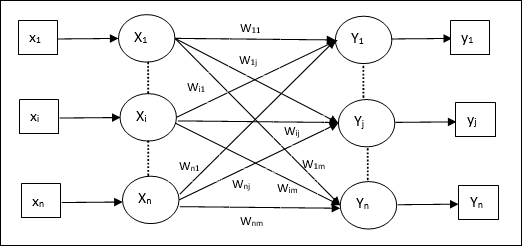
This is a single layer neural network in which the input training vector and the output target vectors are the same. The weights are determined so that the network stores a set of patterns.

Architecture

As shown in the following figure, the architecture of Auto Associative memory network has ‘n’ number of input training vectors and similar ‘n’ number of output target vectors.

Training Algorithm

For training, this network is using the Hebb or Delta learning rule.

Step 1 − Initialize all the weights to zero as w_ij = 0 (i = 1 to n, j = 1 to n)

Step 2 − Perform steps 3-4 for each input vector.

Step 3 − Activate each input unit as follows −

$$x_{i}\:=\:s_{i}\:(i\:=\:1\:to\:n)$$

Step 4 − Activate each output unit as follows −

$$y_{j}\:=\:s_{j}\:(j\:=\:1\:to\:n)$$

Step 5 − Adjust the weights as follows −

$$w_{ij}(new)\:=\:w_{ij}(old)\:+\:x_{i}y_{j}$$

Testing Algorithm

Step 1 − Set the weights obtained during training for Hebb’s rule.

Step 2 − Perform steps 3-5 for each input vector.

Step 3 − Set the activation of the input units equal to that of the input vector.

Step 4 − Calculate the net input to each output unit j = 1 to n

$$y_{inj}\:=\:\displaystyle\sum\limits_{i=1}^n x_{i}w_{ij}$$

Step 5 − Apply the following activation function to calculate the output

$$y_{j}\:=\:f(y_{inj})\:=\:\begin{cases}+1 & if\:y_{inj}\:>\:0\\-1 & if\:y_{inj}\:\leqslant\:0\end{cases}$$

Hetero Associative memory

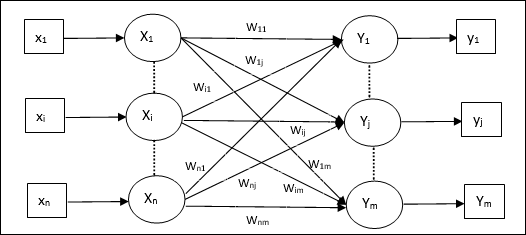
Similar to Auto Associative Memory network, this is also a single layer neural network. However, in this network the input training vector and the output target vectors are not the same. The weights are determined so that the network stores a set of patterns. Hetero associative network is static in nature, hence, there would be no non-linear and delay operations.

Architecture

As shown in the following figure, the architecture of Hetero Associative Memory network has ‘n’ number of input training vectors and ‘m’ number of output target vectors.

Training Algorithm

For training, this network is using the Hebb or Delta learning rule.

Step 1 − Initialize all the weights to zero as w_ij = 0 (i = 1 to n, j = 1 to m)

Step 2 − Perform steps 3-4 for each input vector.

Step 3 − Activate each input unit as follows −

$$x_{i}\:=\:s_{i}\:(i\:=\:1\:to\:n)$$

Step 4 − Activate each output unit as follows −

$$y_{j}\:=\:s_{j}\:(j\:=\:1\:to\:m)$$

Step 5 − Adjust the weights as follows −

$$w_{ij}(new)\:=\:w_{ij}(old)\:+\:x_{i}y_{j}$$

Testing Algorithm

Step 1 − Set the weights obtained during training for Hebb’s rule.

Step 2 − Perform steps 3-5 for each input vector.

Step 3 − Set the activation of the input units equal to that of the input vector.

Step 4 − Calculate the net input to each output unit j = 1 to m;

$$y_{inj}\:=\:\displaystyle\sum\limits_{i=1}^n x_{i}w_{ij}$$

Step 5 − Apply the following activation function to calculate the output

$$y_{j}\:=\:f(y_{inj})\:=\:\begin{cases}+1 & if\:y_{inj}\:>\:0\\0 & if\:y_{inj}\:=\:0\\-1 & if\:y_{inj}\:<\:0\end{cases}$$